Part One got a frame from one device to the next. This part is about going further: the network layer moves packets between networks, and the transport layer delivers their contents to the right process on the right host.
3. The network layer
Services the network layer provides
- Packet forwarding and routing: relays packets between network segments, choosing the most efficient path.
- Connectionless communication (IP): each packet is addressed and routed on its own, as a packet-switched network requires.
- Fragmentation: splits packets that are too large for a link into fragments, which are reassembled at the destination.
Switching techniques
1. Circuit switching
- A dedicated path is set up between the devices for the whole session, and no one else can use it. Common in voice and data communication.
- Advantages: guaranteed bandwidth for the whole call; low latency, because the path is fixed and nothing is set up per packet; predictable performance, with no competition for resources; and a good fit for real-time voice and video.
- Disadvantages: wastes bandwidth, since it is reserved for the whole call; limited scale, since there are only so many circuits; and expensive, because the resources stay dedicated for the call’s duration.
2. Packet switching
- Data is split into packets, each carrying source and destination addresses, and each routed across the network on its own. Packets can arrive out of order, or late when the network is congested.
- Advantages: efficient use of bandwidth, flexibility with different data rates and packet sizes, scales to heavy traffic, and cheap because users share resources.
- Disadvantages: higher latency from passing through many nodes, weak quality-of-service (QoS) guarantees, packets lost to congestion or errors, and so a poor fit for real-time voice and video.
3. Message switching
The notes list this one without detail. In message switching there is no dedicated path and the data is not cut into packets: each node receives the whole message, stores it, and forwards it to the next node when a link is free (store and forward). It needs no setup, but every node needs enough storage for complete messages and the delays are long, so packet switching replaced it. Early telegraph and email relay systems worked this way.
IPv4
- IPv4 (Internet Protocol version 4) was introduced on ARPANET in 1983.
- An IPv4 address is a 32-bit integer, so the address space is 2³² addresses, usually written in dotted-decimal (or hexadecimal) notation.
- In dotted decimal each of the four parts is 0 to 255, written without leading zeros.
- The parts of an IPv4 address:
- Network part: identifies the network, and in classful addressing its class.
- Host part: identifies the machine on that network.
- Subnet number: a network with many hosts is divided into subnets, each given a subnet number.
IP addressing
1. Classful addressing
- On a network, every host ID must be unique. The network address has all host-ID bits set to 0 and names the network; the broadcast address has all host-ID bits set to 1 and reaches every host on it.
- Classful addressing divides the 32-bit space into five classes:
| Class | Leading bits | Network ID bits | Host ID bits | Networks | Addresses per network | Default mask | Range | Purpose |
|---|---|---|---|---|---|---|---|---|
| A | 0 |
8 | 24 | 2⁷ − 2 (126) | 2²⁴ − 2 | 255.0.0.0 | 1.0.0.0 – 126.255.255.255 | Networks with very many hosts |
| B | 10 |
16 | 16 | 2¹⁴ | 2¹⁶ − 2 | 255.255.0.0 | 128.0.0.0 – 191.255.255.255 | Medium to large networks |
| C | 110 |
24 | 8 | 2²¹ | 2⁸ − 2 (254) | 255.255.255.0 | 192.0.0.0 – 223.255.255.255 | Small networks |
| D | 1110 |
– | – | – | – | – | 224.0.0.0 – 239.255.255.255 | Multicast |
| E | 1111 |
– | – | – | – | – | 240.0.0.0 – 255.255.255.255 | Experimental / research |
Notes per class:
- A: 0.x.x.x and 127.x.x.x are special. 127.0.0.0 to 127.255.255.255 is reserved for loopback, used to test networking on the local machine. 0.0.0.0/8 means “this network”: it is used as a source address by a host that does not know its address yet (as in DHCP).
- B: APIPA (Automatic Private IP Addressing) lets a device give itself a link-local address in 169.254.0.0 to 169.254.255.255 when no DHCP server answers.
- C: TEST-NET ranges are reserved for testing and documentation: 192.0.2.0/24, 198.51.100.0/24 and 203.0.113.0/24.
- D: multicast addresses have no network and host parts; they identify multicast groups.
- E: reserved for future and experimental use, not for public use.
On a bit ruler (0, 8, 16, 24, 32), the leading bits fix the class and the rest splits into network and host:
| Class | Bits 1–8 | Bits 9–16 | Bits 17–24 | Bits 25–32 |
|---|---|---|---|---|
| A | 0 + 7 network bits |
host | host | host |
| B | 10 + 6 network bits |
network | host | host |
| C | 110 + 5 network bits |
network | network | host |
| D | 1110 + 4 bits |
multicast group address (28 bits in all) | ||
| E | 1111 + 4 bits |
experimental (28 bits in all) |
2. Classless addressing
Why classless addressing was adopted:
- Reason 1: classful addressing hands out fixed-size blocks, which wastes addresses. Classless addressing assigns a block of whatever size the customer needs.
- Reason 2: addresses had to be shared out fairly among organisations, and internet service providers (ISPs) needed variable-size blocks for their different customers.
CIDR notation:
- A classless address is split into a prefix (the network ID) and a suffix (the host).
- All addresses in a block share the prefix; each host in the block has a different suffix.
- The prefix length n can be anything from 0 to 32, and the suffix is 32 − n bits.
- The prefix length is written after the address with a slash: CIDR (Classless Inter-Domain Routing) notation.
- In 167.199.170.82/27, the prefix is 27 bits, so the suffix is 32 − 27 = 5 bits.
Rules for a CIDR block:
- The addresses in a block must be contiguous.
- The number of addresses must be a power of 2.
- The first address must be divisible by the number of addresses in the block.
Formulas:
- Number of addresses in a block: N = 2^(32 − n), where n is the prefix length.
- First address = (any address in the block) AND (network mask)
- Last address = (any address in the block) OR (NOT network mask)
Example: 167.199.170.82/27
- A /27 prefix means 2⁵ = 32 addresses in the block.
- First address, by ANDing with the mask:
| Binary | Decimal | |
|---|---|---|
| Address | 10100111 11000111 10101010 01010010 |
167.199.170.82 |
| Mask (/27) | 11111111 11111111 11111111 11100000 |
255.255.255.224 |
| AND = first address | 10100111 11000111 10101010 01000000 |
167.199.170.64 |
- Last address, by ORing with the inverted mask:
| Binary | Decimal | |
|---|---|---|
| Address | 10100111 11000111 10101010 01010010 |
167.199.170.82 |
| NOT mask | 00000000 00000000 00000000 00011111 |
0.0.0.31 |
| OR = last address | 10100111 11000111 10101010 01011111 |
167.199.170.95 |
- The block runs from 167.199.170.64 to 167.199.170.95: 32 contiguous addresses, a power of 2, and 64 is divisible by 32, so it satisfies all three rules.
IPv4 header
The header is 20 bytes without options and at most 60 bytes, laid out in 32-bit rows:
| Field | Bits | Meaning |
|---|---|---|
| Version | 4 | IP version: 4 for IPv4 |
| HLEN | 4 | Header length in 32-bit words: minimum 5 (20 bytes), maximum 15 (60 bytes) |
| Type of service | 8 | Requested handling: low delay, high throughput, reliability |
| Total length | 16 | Header plus data, 20 to 65,535 bytes |
| Identification | 16 | Packet ID shared by all fragments of one datagram |
| Flags | 3 | Reserved bit (must be 0), Don’t Fragment (DF), More Fragments (MF) |
| Fragment offset | 13 | Where this fragment’s data sits in the original datagram, in units of 8 bytes (maximum 65,528 bytes) |
| Time to live | 8 | Hop limit: each router decrements it, and the packet is dropped at 0, so it cannot loop forever |
| Protocol | 8 | Which protocol the payload goes to (e.g. 6 = TCP, 17 = UDP) |
| Header checksum | 16 | Error check over the header only |
| Source IP address | 32 | Sender’s address |
| Destination IP address | 32 | Receiver’s address |
| Options | 0–320 (0–40 bytes) | Optional extras such as source route or record route, used by administrators to check whether a path works |
Unicast, broadcast and multicast
-
Unicast: one sender to one receiver, each with its own IP address. One-to-one.
flowchart LR subgraph NA[Network A] A1[Host] end subgraph NB[Network B] B1[Host] end A1 -->|one packet, one receiver| B1 classDef gateway fill:#EDE9FE,stroke:#7C3AED,color:#4C1D95,stroke-width:2px class A1,B1 gateway - Broadcast (one to all), in two forms:
-
Limited broadcast: sent to 255.255.255.255, it reaches every device on the sender’s own network.
flowchart LR S[Sender] --> H1[Host] S --> H2[Host] S --> H3[Host] S --> H4[Host] S --> H5[Host] classDef gateway fill:#EDE9FE,stroke:#7C3AED,color:#4C1D95,stroke-width:2px classDef flow fill:#F1F5F9,stroke:#475569,color:#0F172A,stroke-width:2px class S gateway class H1,H2,H3,H4,H5 flow -
Directed broadcast: a host on one network sends to every host on another network, by setting all the host-ID bits of the destination address to 1 (e.g. 192.168.20.255 for 192.168.20.0/24).
flowchart LR
    subgraph NA[Network A]
        S[Sender]
    end
    subgraph NB[Network B]
        H1[Host]
        H2[Host]
        H3[Host]
        H4[Host]
    end
    S --> H1
    S --> H2
    S --> H3
    S --> H4
    classDef gateway fill:#EDE9FE,stroke:#7C3AED,color:#4C1D95,stroke-width:2px
    classDef flow    fill:#F1F5F9,stroke:#475569,color:#0F172A,stroke-width:2px
    class S gateway
    class H1,H2,H3,H4 flow
-
- Multicast: between unicast and broadcast. One or more senders reach a group of receivers that have joined: the server sends one stream and the network copies it to each member. It uses IGMP (Internet Group Management Protocol), multicast routing, and the class D addresses.
IPv6
- IPv6 was developed by the IETF as the answer to IPv4 address exhaustion. Addresses are 128 bits, a space of 2¹²⁸, written in hexadecimal as 8 groups of 16 bits separated by colons.
- Leading zeros in a group can be dropped, and one run of all-zero groups can be replaced by
:::
| Form | Address |
|---|---|
| Full | 2001:0df8:00f2:0000:0000:0000:0000:0f11 (groups 1–8) |
| Groups 4 to 7 are all zeros, so compress them | 2001:0df8:00f2::0f11 (groups 1, 2, 3 and 8) |
- IPv6 has a more efficient header with options moved out into separate headers, new features and room for extension, support for resource allocation and real-time traffic, and built-in security options for encryption and authentication.
- Addressing methods:
- Unicast: identifies one network interface; packets go to that interface.
- Multicast: identifies a group of hosts; packets go to every member at once.
- Anycast: assigned to a group of interfaces, but a packet goes to only one of them, normally the nearest.
IPv6 has no broadcast addresses.
IPv6 header
A fixed 40-byte header, followed by optional extension headers and then the payload:
| Field | Bits | Meaning |
|---|---|---|
| Version | 4 | IP version: 0110 (6) |
| Traffic class | 8 | Priority, so routers can treat traffic by class. In the original scheme, 0–7 was for congestion-controlled traffic and 8–15 for traffic that is not, typically audio and video. The source sets it and routers may change it. |
| Flow label | 20 | Marks packets of the same flow so routers can handle them the same way; a source and destination can have several flows. |
| Payload length | 16 | Size of everything after the fixed header, extension headers included. Above 65,535 bytes it is set to 0 and the jumbo-payload option is used. |
| Next header | 8 | Type of the first extension header, or of the upper-layer protocol (TCP, UDP) if there is none. |
| Hop limit | 8 | Like IPv4’s TTL: decremented by each router, packet discarded at 0. |
| Source address | 128 | The original sender. |
| Destination address | 128 | The final destination, used by routers on the way. |
Extension headers replace IPv4’s options field. The next-header field points to the first one, and each points to the next, forming a chain.
Routing
Routing is what layer 3 devices do: choose the best path to deliver a packet from one network to another.
Types of routing
- Static routing
- Routes are added to the routing table by hand.
- Advantages: no routing work for the router’s CPU, more security because the router only routes to the networks it is told about, and no bandwidth spent between routers.
- Disadvantages: in a large network an administrator must add routes on every router by hand, and needs to know the whole topology.
An example topology, with a static route on each router for every network it is not directly connected to:
flowchart LR LAN3["LAN 10.10.10.0/24"] --- R3[R3] R3 ---|"s0/0 172.16.10.1/30 ↔ s0/0/0 172.16.10.2/30"| R2[R2] R3 ---|"s0/1 172.16.10.5/30 ↔ s0/0/1 172.16.10.6/30"| R1[R1] R2 --- LAN2["LAN 192.168.10.0/24 + PC"] R1 --- LAN1["LAN 192.168.20.0/24 + PC"] classDef gateway fill:#EDE9FE,stroke:#7C3AED,color:#4C1D95,stroke-width:2px classDef store fill:#CFFAFE,stroke:#0891B2,color:#164E63,stroke-width:2px class R1,R2,R3 gateway class LAN1,LAN2,LAN3 store - Default routing
- Every packet goes to one configured next-hop router, whatever the destination. Used on stub routers, which have only one way out to all other networks.
- Dynamic routing
- Routers exchange route information with protocols such as RIP and OSPF, and adjust their tables as the topology changes.
- Easy to configure, picks good routes and discovers remote networks, but it uses more bandwidth talking to neighbours and is less secure than static routing.
Routing protocols
1. Intra-domain (interior gateway) protocols
Distance vector routing (DVR)
- Each router periodically tells its neighbours its distances to every destination.
- Also known as the old ARPANET routing algorithm, or the Bellman-Ford algorithm.
- The algorithm:
- A router sends its distance vector to each neighbour in a routing packet.
- Each router saves the latest distance vector from each neighbour.
- A router recalculates its own vector when:
- a neighbour sends a vector with different information than before, or
- it finds that the link to a neighbour has gone down.
Example. Three routers with link costs X–Y = 1, Y–Z = 2 and X–Z = 5. At first each router knows only its own direct links:
| From | to X | to Y | to Z |
|---|---|---|---|
| X | 0 | 1 | 5 |
| Y | 1 | 0 | 2 |
| Z | 5 | 2 | 0 |
X receives Y’s vector and sees that X → Y → Z costs 1 + 2 = 3, less than the direct 5, so it updates its route to Z to 3 via Y. Z does the same for its route to X. Once the vectors have been exchanged, every router holds the same, converged table:
| From | to X | to Y | to Z |
|---|---|---|---|
| X | 0 | 1 | 3 (via Y) |
| Y | 1 | 0 | 2 |
| Z | 3 (via Y) | 2 | 0 |
Routing Information Protocol (RIP)
- Uses hop count as its metric for the best path. Runs on UDP port 520.
- Hop count is the number of routers between source and destination. RIP caps it to prevent routing loops: the maximum is 15, and 16 means “network unreachable”.
- Features: routers exchange updates periodically, broadcast (or multicast) them, send their whole routing table each time, and trust what their neighbours say, which is why it is called routing on rumours.
- RIP versions:
| RIP v1 | RIP v2 | RIPng |
|---|---|---|
| Updates are broadcast | Updates are multicast | Updates are multicast |
| Broadcast to 255.255.255.255 | Multicast to 224.0.0.9 | Multicast to FF02::9 (RIPng runs only on IPv6) |
| No authentication of updates | Supports authentication of updates | – |
| Classful | Classless | Classless |
- Common in small and medium networks, legacy networks and labs. Easy to configure, needs little maintenance, and serves as a backup routing protocol in some networks.
- Advantages: simple, easy to implement, automatic updates, low overhead in a small network, works with most devices.
- Limitations: poor scalability, slow convergence (the notes list both fast and slow; slow is right for large networks), routing loops, little load-balancing support, security weaknesses, and wasted bandwidth from sending full tables.
Link state routing
- Routers exchange messages to learn the whole network topology, then compute their routing tables with a shortest-path calculation.
- Each router floods link-state packets describing its links. Together they form a link-state database, on which each router runs shortest path first (Dijkstra’s algorithm) to build its routing table of paths and interfaces.
Example. The network, with link costs:
flowchart LR
    A((A)) ---|4| B((B))
    A ---|8| C((C))
    B ---|8| D((D))
    B ---|11| C
    C ---|7| E((E))
    C ---|1| F((F))
    D ---|2| E
    D ---|7| G((G))
    D ---|4| H((H))
    E ---|6| F
    F ---|2| H
    G ---|14| H
    G ---|9| I((I))
    H ---|10| I
    classDef gateway fill:#EDE9FE,stroke:#7C3AED,color:#4C1D95,stroke-width:2px
    class A,B,C,D,E,F,G,H,I gateway
Dijkstra from A: at each step, fix the closest node not yet fixed, then update its neighbours’ tentative distances.
| Step | Fixed (shortest distance known) | Tentative distances |
|---|---|---|
| 1 | A 0 | B 4, C 8 |
| 2 | A 0, B 4 | C 8, D 12 (via B) |
| 3 | A 0, B 4, C 8 | D 12, E 15 (via C), F 9 (via C) |
| 4 | … F 9 | D 12, E 15 (via F), H 11 (via F) |
| 5 | … H 11, D 12 | E 14 (via D), G 19 (via D), I 21 (via H) |
| Final | A 0, B 4, C 8, D 12, E 14, F 9, G 19, H 11, I 21 | – |
The resulting shortest-path tree from A:
flowchart LR
    A((A 0)) -->|4| B((B 4))
    A -->|8| C((C 8))
    B -->|8| D((D 12))
    C -->|1| F((F 9))
    F -->|2| H((H 11))
    D -->|2| E((E 14))
    D -->|7| G((G 19))
    H -->|10| I((I 21))
    classDef ok fill:#DCFCE7,stroke:#16A34A,color:#14532D,stroke-width:2px
    class A,B,C,D,E,F,G,H,I ok
Open Shortest Path First (OSPF)
- A link-state protocol: routers exchange topology information with their neighbours and compute end-to-end paths with a variant of Dijkstra’s algorithm.
- Its main strength is that routes can be computed against specific criteria, which is useful for traffic engineering and quality of service.
- Its main weakness is scaling: as routers are added, topology updates get larger and more frequent and route calculation takes longer. (OSPF areas are the standard way to contain this.)
- Each router describes its local state in link-state advertisements (LSAs), from which every router builds an identical topology database.
- From the database, each router computes its routing table with the SPF algorithm: destinations, next-hop IP addresses and outgoing interfaces.
- It recalculates routes when the topology changes, and keeps routing traffic to a minimum.
Enhanced Interior Gateway Routing Protocol (EIGRP)
- A dynamic routing protocol that finds the best path between layer 3 devices using a composite metric. It runs directly over IP as protocol number 88.
- EIGRP talks to its neighbours with these messages:
- Hello: exchanged to discover or recover neighbours and check that a device runs EIGRP. They carry the AS number and the k values. Hellos can be multicast or unicast, and a hello with no data doubles as an acknowledgement.
- Null update: used to compute the smooth round-trip timer (SRTT), the time for a packet to reach the neighbour and be acknowledged, and the retransmission timeout (RTO), how long to wait for an acknowledgement when multicast fails.
- Full update: exchanged once neighbours are formed, carrying all best routes.
- Partial update: sent when the topology changes or links are added; only new routes, and multicast.
- Query: multicast when a route is lost and there is no alternative in the topology table.
- Reply: answers a query with a route to the requested network.
- Acknowledgement: acknowledges updates, queries and replies.
Hello and acknowledgement packets are not acknowledged. Updates, queries and replies are reliable and must be.
2. Inter-domain (exterior gateway) protocols
Border Gateway Protocol (BGP)
- The internet’s routing protocol between autonomous systems (ASes): it exchanges reachability information so that networks with different internal topologies can reach each other.
- It uses the next-hop paradigm, lets several BGP speakers in one AS coordinate, carries path information in its advertisements, and lets administrators apply custom policies. It runs over TCP for reliable delivery, saves bandwidth by sending incremental updates, supports CIDR, and supports authentication of sessions between peers.
- Three main functions:
- Peer acquisition and authentication: peers open a TCP connection and exchange messages to agree to communicate.
- Sending reachability information: peers exchange both positive and negative information about which routes are available.
- Verifying connectivity: peers check each other and the link between them keep working.
- It also manages route information: storing, updating, selecting and advertising routes.
flowchart LR
    AS1["AS-1<br/>(EIGRP inside)"] <-->|BGP| ISP1["ISP-1<br/>(IS-IS inside)"]
    AS1 <-->|BGP| ISP2["ISP-2<br/>(OSPF inside)"]
    ISP1 <-->|BGP| ISP2
    ISP1 <-->|BGP| AS2["AS-2<br/>(OSPF inside)"]
    ISP2 <-->|BGP| AS2
    ISP2 -->|static route| AS3["AS-3<br/>(RIP inside)"]
    AS3 -->|default static route| ISP2
    classDef gateway fill:#EDE9FE,stroke:#7C3AED,color:#4C1D95,stroke-width:2px
    classDef store   fill:#CFFAFE,stroke:#0891B2,color:#164E63,stroke-width:2px
    class AS1,AS2,AS3 gateway
    class ISP1,ISP2 store
Inside each AS an interior protocol runs; between them, BGP. A small AS with one link to its ISP (AS-3) needs no BGP: a static route in and a default route out are enough.
Network address translation (NAT)
- NAT lets many devices on a private network reach the internet through one public IP address. It rewrites private addresses to public ones on the way out and back on the way in, and also rewrites port numbers. It usually runs on a router or firewall.
- How it works: the border router, configured for NAT, translates local IP addresses to global ones as packets leave the network, and back again as replies come in. If the NAT address pool is exhausted, packets are dropped and an ICMP host unreachable message goes back to the sender.
sequenceDiagram
    participant A as Host A 10.0.0.5:3345
    participant N as NAT router (public 203.0.113.7)
    participant S as Server 93.184.216.34:80
    A->>N: src 10.0.0.5:3345
    Note over N: records 10.0.0.5:3345 ↔ 203.0.113.7:5001
    N->>S: src 203.0.113.7:5001
    S->>N: dst 203.0.113.7:5001
    Note over N: looks up 5001 in the NAT table
    N->>A: dst 10.0.0.5:3345
- Why translate port numbers too?
- Hosts A and B on the network contact the same destination at the same moment, both from the same source port.
- If NAT rewrote only the IP addresses, both would leave with the router’s public IP and the same port.
- Replies come back to the router’s public IP, and NAT could not tell which reply belongs to which host, because the ports are identical.
- So NAT also rewrites the source port, giving each connection a unique one.
- It keeps a NAT table mapping each public port back to the right host.
- Inside and outside addresses:
- Inside local: the address assigned to a host on the inside network, usually a private address rather than one from the ISP. The inside host as seen from inside.
- Inside global: the public address that represents one or more inside local addresses to the outside world. The inside host as seen from outside.
- Outside local: the address of the outside destination host as it appears inside the network, after translation.
- Outside global: the outside host’s real address as seen on the outside network, before translation.
- Types of NAT:
- Static NAT: a fixed one-to-one mapping between a private and a public address. Used for hosting web servers, but expensive when many public addresses are needed.
- Dynamic NAT: private addresses are mapped to public addresses from a pool. Only as many hosts as there are pool addresses can be translated at once, and packets may be dropped when the pool is full. Suits a fixed number of users, but still needs several public addresses.
- PAT (port address translation), or NAT overload: many private addresses share one public address, told apart by port number. Thousands of users can share one public address, so it is cheap, and it is by far the most common type.
- Advantages: saves registered public addresses, gives some privacy by hiding devices’ addresses, and avoids renumbering when the network changes.
- Disadvantages: adds delay on the switching path, breaks some applications, complicates tunnelling protocols such as IPsec, and makes the router handle port numbers, beyond a network layer device’s usual job.
Tunnelling
- Tunnelling connects two networks of one type across an intermediate network of another type. It wraps (encapsulates) packets of one protocol inside packets of another, following a layered model such as OSI or TCP/IP.
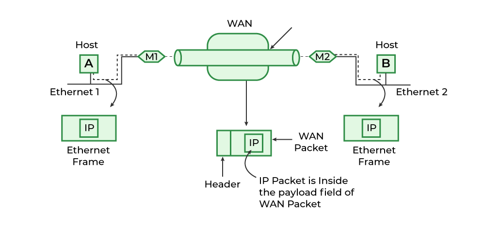
- The WAN becomes one “big tunnel” between the multiprotocol routers M1 and M2, and hosts A and B talk as if it were not there: M1 encapsulates the IP packet inside a WAN packet and M2 takes it out.
- Tunnelling protocols:
- GRE (Generic Routing Encapsulation): wraps an IP packet in a GRE header plus a new delivery header with its own source and destination, hiding the original. The routers at each end add and strip it, so the original packet crosses the tunnel and emerges unchanged. (GRE itself does not encrypt.)
- IPsec (Internet Protocol Security): an IETF protocol suite that secures traffic between two points on an IP network, with data authentication, integrity, confidentiality, and key exchange and management.
- IP-in-IP: encapsulates an IP packet inside another IP packet.
- SSH (Secure Shell): a cryptographic protocol for secure, encrypted transfer over a network, used for remote login (with key-based logins, without typing a password for each system) and for tunnelling other traffic.
- PPTP (Point-to-Point Tunneling Protocol): a long-standing VPN protocol that builds a tunnel and uses PPP (Point-to-Point Protocol) to encrypt packets. Supported on Windows, Mac and Linux (and now considered insecure).
- SSTP (Secure Socket Tunneling Protocol): Microsoft’s VPN protocol, secured with SSL/TLS, mainly on Windows.
- L2TP (Layer 2 Tunneling Protocol): published in 2000 for VPNs over the internet. It combines the best of PPTP and L2F so ISPs can offer VPN services.
- VXLAN (Virtual Extensible LAN): a network virtualisation technology that stretches layer 2 across layer 3 networks by wrapping Ethernet frames in VXLAN packets with IP addresses, which scales further than VLANs.
- What is SSL tunnelling? A client that needs an SSL/TLS connection to a backend service goes through a proxy server. The proxy opens the connection to the backend and then copies bytes in both directions without touching the encrypted SSL session.
sequenceDiagram
    participant C as Client
    participant P as Proxy server :8080
    participant S as Server :443
    C->>P: CONNECT server:443 (request a secure connection)
    P->>S: open a TCP connection to port 443
    P-->>C: connection established
    C->>S: TLS session, relayed byte for byte through the proxy
ARP and RARP
The ARP family:
- Address Resolution Protocol (ARP)
- Finds the MAC address that goes with an IP address on the same network. It works between the network layer and the data-link layer.
- Before sending an IP packet the sender must know the destination’s MAC address. It broadcasts an ARP request, only the machine with that IP answers with a unicast ARP reply, the sender stores the answer in its ARP cache, and from then on sends unicast frames.
sequenceDiagram participant P1 as PC1 participant P2 as PC2 (192.168.1.2) participant P3 as PC3 participant P4 as PC4 P1->>P2: ARP request (broadcast): who has 192.168.1.2? P1->>P3: same broadcast P1->>P4: same broadcast Note over P3,P4: not 192.168.1.2, ignore it P2-->>P1: ARP reply (unicast): 192.168.1.2 is at my MAC Note over P1: stores the mapping in its ARP cache - Reverse ARP (RARP)
- A device that knows its MAC address but not its IP address asks for one. A RARP server on the LAN answers the broadcast by looking the MAC up in its IP-to-MAC table.
- It worked over Ethernet, Ethernet II, Token Ring and FDDI, but is little used today: BOOTP and DHCP do the job better.
sequenceDiagram participant A as Device A (MAC known, IP unknown) participant R as RARP server A->>R: broadcast: my MAC is 210, what is my IP address? R-->>A: your IP address is IPA - Inverse ARP (InARP): finds an IP address from a link-layer identifier in networks such as ATM and Frame Relay. It maps a local identifier (a DLCI) to the remote end’s IP address when the identifier is known but the address is not.
- Proxy ARP: lets devices on different segments of one IP network, separated by a router, reach each other. The router answers ARP requests on the other segment’s behalf with its own MAC address and forwards the traffic, since the broadcast would not cross it.
- Gratuitous ARP: a host announces its own IP-to-MAC mapping, unasked, typically at boot or when its address changes. It detects IP conflicts (someone else answering means the address is taken), and updates other hosts’ ARP caches and switches’ MAC tables.
ARP poisoning (ARP spoofing)
- An attacker on the LAN sends forged ARP messages that tie the attacker’s MAC address to a legitimate device’s IP address.
- Traffic meant for that IP then goes to the attacker, who can read, change or stop it in transit.
- It opens the door to worse attacks: man-in-the-middle, denial of service and session hijacking.
flowchart LR
    Bob["Bob<br/>192.168.0.1 · aa:aa"] <-->|via router| Mary["Mary<br/>192.168.0.5 · bb:bb"]
    Att["Attacker<br/>192.168.0.3 · cc:cc"] -.->|"forged ARP: 192.168.0.5 is at cc:cc"| Bob
    Att -.->|"forged ARP: 192.168.0.1 is at cc:cc"| Mary
    classDef gateway fill:#EDE9FE,stroke:#7C3AED,color:#4C1D95,stroke-width:2px
    classDef error   fill:#FEE2E2,stroke:#DC2626,color:#7F1D1D,stroke-width:2px
    class Bob,Mary gateway
    class Att error
With both caches poisoned, Bob’s and Mary’s traffic to each other flows through the attacker.
ARP vs RARP
| ARP | RARP |
|---|---|
| Maps an IP address to a physical (MAC) address | Maps a physical (MAC) address to an IP address |
| Finds the MAC of a device whose IP is known | Finds the IP of a device whose MAC is known |
| The client broadcasts an IP address and asks for the MAC | The client broadcasts its MAC and asks for an IP |
| The owner of the IP answers with its MAC | The RARP server answers with the IP |
| Used everywhere in modern networks | Rarely used; devices get IPs from DHCP |
| Each host keeps its own ARP table | The RARP server keeps the RARP table |
| Fetches the receiver’s MAC address | Fetches the device’s own IP address |
| ARP replies update the ARP table | RARP replies configure the IP address |
| Used by hosts and routers to find MAC addresses | Used by small, diskless machines |
| Used on the sender’s side to map the receiver’s MAC | Used on the requesting side to learn its own IP |
4. The transport layer
How the transport layer works
- At the sender: it takes the message from the application layer and segments it, adds the source and destination port numbers to each segment’s header, and hands the segments to the network layer.
- At the receiver: it takes data from the network layer, reassembles the segments, reads the header, finds the port number, and passes the message to the right application.
Responsibilities of the transport layer
1. Process-to-process delivery
- The data-link layer needs MAC addresses to deliver a frame; the network layer needs IP addresses to route a packet.
- In the same way, the transport layer needs a port number to deliver a segment to the right process among the many running on a host.
- A port number is a 16-bit address that identifies a program on a host.
flowchart LR
    subgraph H1[Host 1]
        P1["Browser :50514"]
    end
    subgraph H2[Host 2]
        W["Web server :443"]
        M["Mail server :25"]
    end
    P1 -->|"MAC: next device · IP: host 2 · port: 443"| W
    classDef gateway fill:#EDE9FE,stroke:#7C3AED,color:#4C1D95,stroke-width:2px
    classDef flow    fill:#F1F5F9,stroke:#475569,color:#0F172A,stroke-width:2px
    class P1,W gateway
    class M flow
2. End-to-end connection between hosts
- The transport layer creates the end-to-end connection between hosts, mainly with TCP and UDP.
- TCP is a reliable, connection-oriented protocol. It sets up the connection with a handshake and guarantees delivery.
- UDP is stateless and unreliable: best-effort delivery. It suits applications that care little about flow and error control and send a lot of data, such as video conferencing, and it is often used for multicast.
flowchart LR
    E1([End system]) --- R1[Router] --- R2[Router] --- R3[Router] --- E2([End system])
    E1 -.->|end-to-end connection: only the end systems run TCP or UDP| E2
    classDef actor fill:#DBEAFE,stroke:#2563EB,color:#1E3A8A,stroke-width:2px
    classDef flow  fill:#F1F5F9,stroke:#475569,color:#0F172A,stroke-width:2px
    class E1,E2 actor
    class R1,R2,R3 flow
3. Multiplexing and demultiplexing
- Multiplexing (many to one): at the sender, data from several processes is gathered, given headers, and sent over one network connection.
- It lets many processes on a host use the network at once, told apart by their port numbers.
- Demultiplexing (one to many): at the receiver, incoming segments are handed out to the right processes.
- The transport layer takes segments from the network layer and demultiplexes them, delivering each to the process it is addressed to.
flowchart LR
    subgraph Src[Source]
        Y1[Yahoo] --> Mux[Multiplexing]
        G1[Gmail] --> Mux
        O1[Outlook] --> Mux
    end
    Mux -->|"segments: Yahoo · Gmail · Outlook · Gmail · Yahoo"| Dmx[Demultiplexing]
    subgraph Dst[Destination]
        Dmx --> Y2[Yahoo]
        Dmx --> G2[Gmail]
        Dmx --> O2[Outlook]
    end
    classDef warn    fill:#FEF3C7,stroke:#D97706,color:#78350F,stroke-width:2px
    classDef gateway fill:#EDE9FE,stroke:#7C3AED,color:#4C1D95,stroke-width:2px
    class Mux,Dmx warn
    class Y1,G1,O1,Y2,G2,O2 gateway
4. Congestion control
- Congestion happens when too many sources send at once: router buffers overflow, packets are lost, and they have to be retransmitted.
Congestion control algorithms:
- Leaky bucket
- When a host wants to send a packet, it drops it into the bucket.
- The bucket leaks at a constant rate: the interface transmits at a fixed rate.
- Bursty traffic comes out as smooth, uniform traffic.
- In practice the bucket is a finite queue emptied at a fixed rate.
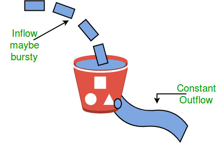
Bursty in, constant out. - Token bucket
- A more flexible alternative to the leaky bucket for traffic shaping and rate limiting.
- Tokens are added to the bucket at a fixed rate, one every tick, and each packet must take a token to be sent. When tokens have built up, a burst of packets can go out at once.
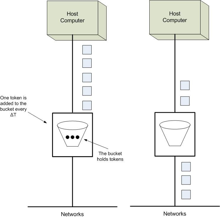
(A) The bucket holds 3 tokens and 5 packets wait. (B) 3 packets were sent; 2 wait for more tokens.
TCP congestion control
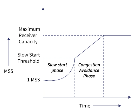
TCP keeps a congestion window (cwnd) as well as the receiver’s window, so both the receiver and the network limit how much the sender has in flight. It moves through three phases:
-
Slow start: cwnd starts at 1 MSS (maximum segment size) and grows by 1 MSS for every acknowledgement, which doubles it every round trip: exponential growth. cwnd = cwnd + MSS (per ACK).
After round trip Congestion window Result 1 2¹ 2 MSS 2 2² 4 MSS 3 2³ 8 MSS sequenceDiagram participant S as Sender participant R as Receiver Note over S: cwnd = 1 MSS S->>R: segment 1 R-->>S: ack Note over S: cwnd = 2 MSS S->>R: segments 1–2 R-->>S: acks 1–2 Note over S: cwnd = 4 MSS S->>R: segments 1–4 R-->>S: acks 1–4 Note over S: cwnd = 8 MSS - Congestion avoidance: once cwnd reaches the slow-start threshold, it grows linearly: by 1 MSS per round trip (in practice MSS × MSS / cwnd per acknowledgement, which adds up to one MSS per round trip). It keeps growing until it reaches the receiver’s window size.
- Congestion detection: the sender reacts to a lost segment according to how it found out:
- Timeout: the timer expires before the acknowledgement arrives. This is the stronger sign
of congestion; a segment has probably been dropped. Reaction:
- set the threshold to half the current window,
- drop cwnd to 1 MSS,
- go back to slow start.
- Three duplicate acknowledgements: the weaker sign. One segment was probably lost while
later ones got through. Reaction:
- set the threshold to half the current window,
- set cwnd to the new threshold,
- continue in congestion avoidance.
- Timeout: the timer expires before the acknowledgement arrives. This is the stronger sign
of congestion; a segment has probably been dropped. Reaction:
5. Data integrity and error correction
- The transport layer checks application data for errors with error-detection codes and checksums, verifies it is not corrupted, and uses ACK (acknowledgement) and NACK (negative acknowledgement) to tell the sender whether it arrived. The checksum works as in Part One: the sender adds the n-bit subunits, complements the sum and sends it with the data; the receiver adds everything, complements, and a result of 0 means no error.
flowchart LR
    subgraph Sender
        direction TB
        S1[Subunits 1..k, n bits each] --> S2[Sum] --> S3[Complement = checksum]
    end
    subgraph Receiver
        direction TB
        R1[Subunits + checksum] --> R2[Sum] --> R3[Complement] --> R4{Zero?}
    end
    S3 -->|data + checksum| R1
    R4 -->|yes| OK([No error])
    R4 -->|no| ER([Error])
    classDef flow  fill:#F1F5F9,stroke:#475569,color:#0F172A,stroke-width:2px
    classDef warn  fill:#FEF3C7,stroke:#D97706,color:#78350F,stroke-width:2px
    classDef ok    fill:#DCFCE7,stroke:#16A34A,color:#14532D,stroke-width:2px
    classDef error fill:#FEE2E2,stroke:#DC2626,color:#7F1D1D,stroke-width:2px
    class S1,S2,S3,R1,R2,R3 flow
    class R4 warn
    class OK ok
    class ER error
Error control in TCP
- TCP detects corrupted, missing, out-of-order and duplicated segments.
- It does so with three simple mechanisms:
- Checksum: every segment carries one. A corrupted segment is discarded by the receiver and treated as lost.
- Acknowledgement: confirms that data segments arrived. Control segments that carry no data but consume sequence numbers (SYN, FIN) are acknowledged too; pure ACK segments are not.
- Retransmission: a missing, delayed or corrupted segment is sent again, either when a
timer runs out or when three duplicate ACKs arrive:
- After RTO: TCP keeps a retransmission timeout (RTO) timer for unacknowledged segments. When it expires, the earliest one is resent. The RTO is updated continually from measured round-trip times.
- After three duplicate ACKs (fast retransmit): if the RTO is long, three duplicate ACKs trigger an immediate resend of the missing segment instead of waiting for the timer.
6. Flow control
- TCP stops a fast sender from overrunning a slow receiver, so no data is lost to the speed difference. It uses a sliding window: the receiver tells the sender how much it can accept, and the sender never has more than that outstanding.
Port numbers
- A port number is a 16-bit integer, 0 to 65,535.
- Servers listen on well-known ports, 0 to 1023, which are privileged.
- Clients use ephemeral (short-lived) ports.
- The Internet Assigned Numbers Authority (IANA) keeps the list of assignments:
- Well-known ports (0–1023) are controlled and assigned by IANA.
- Registered ports (1024–49151) are registered with IANA for convenience. 49151 is about three quarters of the 65,536 possible ports.
- Dynamic ports (49152–65535) are the ephemeral ports.
Sockets
- A socket is one endpoint of a two-way communication link between two programs on a network.
- Its address is an IP address plus a port number.
- It enables inter-process communication (IPC) by giving each side a named point of contact.
- It is created with the
socketsystem call, much aspipecreates a pipe. - It gives bidirectional FIFO communication over the network.
- Sockets are the basis of client-server applications:
- The server creates a socket, binds it to a port and waits for clients.
- The client creates a socket and connects it to the server’s socket.
- Once the connection is up, data flows.
flowchart LR
    X["host X 146.86.5.20<br/>socket 146.86.5.20:1625"] <-->|connection| W["web server 161.25.19.8<br/>socket 161.25.19.8:80"]
    classDef gateway fill:#EDE9FE,stroke:#7C3AED,color:#4C1D95,stroke-width:2px
    class X,W gateway
- Types of socket:
- Datagram socket: connectionless, like a mailbox: packets posted to it are collected and delivered to the receiving socket.
- Stream socket: connection-oriented, a sequenced flow of bytes with no record boundaries. Like a phone call: a connection is set up and the two ends talk over it.
- Socket calls:
sequenceDiagram
    participant S as Server
    participant C as Client
    Note over S: socket() → bind() → listen()
    Note over C: socket()
    C->>S: connect()
    Note over S: accept()
    C->>S: send() → recv()
    S->>C: send() → recv()
    C->>S: close()
    Note over S: close()
| Call | What it does |
|---|---|
socket() |
Create a socket |
bind() |
Give the socket an address, like a phone number to be reached on |
listen() |
Get ready to accept connections |
connect() |
Connect to a listening socket, as the caller |
accept() |
Accept an incoming connection, like answering a call |
write() / send() |
Send data |
read() / recv() |
Receive data |
close() |
Close the connection |
TCP
- TCP (Transmission Control Protocol) is a reliable, connection-oriented protocol that delivers data securely and in order across interconnected networks, in full duplex.
- Advantages: reliable, with error checking and recovery; flow control; delivery and order are guaranteed; it is an open protocol owned by no one; and, as part of the TCP/IP suite, it works with IP addressing and domain names so hosts can be told apart.
- Disadvantages: heavyweight for small networks with few resources, its several layers can slow things down, it belongs to the TCP/IP suite and cannot run on other stacks such as Bluetooth’s, and its core design has changed little since it was created decades ago.
Sequence and acknowledgement numbers
- Byte number: every byte to be sent is numbered, starting from an arbitrary value.
- Sequence number: a segment’s sequence number is the byte number of its first byte, so the receiver can put segments back in order even if they arrive out of order.
- Acknowledgement number: because TCP is full duplex, each side also acknowledges. The acknowledgement number is the next byte the receiver expects, which confirms every byte before it.
sequenceDiagram
    participant A as Host A
    participant B as Host B
    A->>B: Seq 12001, Ack 1001, bytes 12001–13001
    B->>A: Seq 1001, Ack 13002, bytes 1001–2001
A’s acknowledgement 1001 says it has everything up to byte 1000 and expects 1001 next. B’s acknowledgement 13002 says it has received A’s bytes up to 13001 and expects 13002 next.
TCP header
20 to 60 bytes, followed by the data:
| Field | Bits | Meaning |
|---|---|---|
| Source port | 16 | Port of the sending application |
| Destination port | 16 | Port of the receiving application |
| Sequence number | 32 | Byte number of the first data byte in this segment, for reassembly |
| Acknowledgement number | 32 | The next byte the receiver expects, acknowledging everything before it |
| Header length (HLEN) | 4 | Header length in 4-byte words: 5 (20 bytes, the minimum) to 15 (60 bytes, the maximum) |
| Reserved | 6 | Unused |
| Control flags | 6 | URG, ACK, PSH, RST, SYN, FIN (below) |
| Window size | 16 | How many bytes the sender of this segment can receive |
| Checksum | 16 | Error check; mandatory in TCP, unlike UDP |
| Urgent pointer | 16 | Valid only with URG: added to the sequence number, gives the byte number of the last urgent byte |
| Options and padding | 0–320 (0–40 bytes) | Extras such as MSS and window scaling |
The six flags control setting up, tearing down and aborting connections, flow control and how data is handed over:
- URG: the urgent pointer is valid.
- ACK: the acknowledgement number is valid.
- PSH: push the data to the application now.
- RST: reset the connection.
- SYN: synchronise sequence numbers.
- FIN: finish (close) the connection.
The three-way handshake
- TCP uses positive acknowledgement with retransmission (PAR): receipt is confirmed with acknowledgements, and anything lost or corrupted is sent again.
- The transport layer’s PDU (protocol data unit) is the segment.
- A damaged segment fails its checksum and is discarded by the receiver.
- The sender keeps retransmitting until it gets a positive acknowledgement.
- Three segments are exchanged to set up a connection:
- Step 1 (SYN): the client sends a segment with SYN set, telling the server it wants to talk and what sequence number it will start from.
- Step 2 (SYN + ACK): the server replies with both flags set: ACK acknowledges the client’s segment, and SYN gives the sequence number the server will start from.
- Step 3 (ACK): the client acknowledges the server’s reply. The connection is up and data transfer can start.
sequenceDiagram
    participant C as Client
    participant S as Server
    C->>S: SYN (seq = m)
    S->>C: SYN + ACK (seq = n, ack = m + 1)
    C->>S: ACK (ack = n + 1)
    Note over C,S: connection established
Connection establishment, with real numbers
- The sender opens with:
- Seq = 521: its random initial sequence number (RISN).
- SYN = 1: asks the receiver to synchronise with that sequence number.
- MSS = 1460 B: its maximum segment size, so segments will not need fragmenting.
- Window = 14600 B: how much it can buffer from the receiver.
- The receiver replies with:
- Seq = 2000: its own random initial sequence number.
- SYN = 1: asks the sender to synchronise with it.
- MSS = 500 B: its maximum segment size; the two sides use the smaller.
- Window = 10000 B: how much it can buffer from the sender.
- Ack = 522: acknowledges the SYN and asks for byte 522 next.
- ACK = 1: the acknowledgement number is valid.
- The sender finishes with:
- Seq = 522: the next sequence number.
- Ack = 2001: acknowledges the receiver’s SYN and asks for byte 2001 next.
- ACK = 1.
sequenceDiagram
    participant S as Sender (RISN 521)
    participant R as Receiver (RISN 2000)
    S->>R: Seq 521, SYN 1, MSS 1460 B, window 14600 B
    R->>S: Seq 2000, SYN 1, MSS 500 B, window 10000 B, Ack 522, ACK 1
    S->>R: Seq 522, Ack 2001, ACK 1
    Note over S,R: data transfer
A SYN consumes 1 sequence number, a bare ACK consumes 0, and every data byte consumes 1. That is why the acknowledgements are 522 and 2001 even though no data has been sent.
Connection termination
TCP releases connections in two ways:
- Graceful release: the connection stays open until both sides have closed their half.
- Abrupt release: one side is forced to close, or one user closes both directions at once.
Abrupt release with RST (reset). An RST segment is sent when:
- a segment other than SYN arrives for a connection that does not exist;
- a segment arrives with an invalid header, to fend off attacks;
- there are not enough resources for the connection, or the remote host is unreachable.
Graceful release with FIN. The notes’ version of this sequence had the states tangled; here it is as TCP defines it:
- The client (the side closing first) sends a segment with FIN set and enters FIN_WAIT_1.
- The server acknowledges it with an ACK and enters CLOSE_WAIT. The client, on getting the ACK, enters FIN_WAIT_2. Data can still flow from server to client.
- When the server is done, it sends its own FIN and enters LAST_ACK.
- The client acknowledges that FIN and enters TIME_WAIT. The server, on getting the ACK, closes.
- The client stays in TIME_WAIT for a while (twice the maximum segment lifetime) in case its final ACK was lost and the server’s FIN is retransmitted.
- Then the client closes too and releases its resources.
sequenceDiagram
    participant C as Client (active close)
    participant S as Server (passive close)
    Note over C,S: ESTABLISHED
    C->>S: FIN
    Note over C: FIN_WAIT_1
    S->>C: ACK
    Note over S: CLOSE_WAIT
    Note over C: FIN_WAIT_2
    S->>C: FIN
    Note over S: LAST_ACK
    C->>S: ACK
    Note over C: TIME_WAIT, then CLOSED
    Note over S: CLOSED
Piggybacking
- Piggybacking means holding back an acknowledgement and attaching it to the next outgoing data frame, so the ACK travels with the data instead of on its own.
sequenceDiagram
    participant A as Host A
    participant B as Host B
    A->>B: data
    B->>A: data + ACK for A's data (piggybacked)
    Note over A: nothing left to send
    A->>B: ACK only
- Context: sliding-window algorithms let a sender have several frames unacknowledged at once. Both ends keep finite buffers, timers resend anything unacknowledged, the sender can send a whole window before the first ACK comes back, and the receiver advertises its window so its buffer never overflows.
- Raising efficiency: full-duplex transmission lets both sides send at once, like having two half-duplex links.
- Why piggyback: in full duplex you can either run two separate channels, each carrying data one way and ACKs the other, or piggyback: the receiver waits until it has data of its own to send and carries the ACK on it.
- Advantages: better use of channel bandwidth, lower cost, lower latency, and fewer delays and retransmissions thanks to short timers.
- Disadvantages: more complexity, and if the receiver waits too long to send its acknowledgement, the sender times out and retransmits the frame.
UDP
- UDP (User Datagram Protocol) is a connectionless, unreliable transport protocol in the TCP/IP suite. It is low-latency and tolerates loss, with no connection set up first.
UDP header (8 bytes, followed by the data):
| Field | Bits | Meaning |
|---|---|---|
| Source port | 16 | Port of the sender |
| Destination port | 16 | Port the datagram is for |
| Length | 16 | Length of header plus data |
| Checksum | 16 | One’s complement of the one’s-complement sum of the UDP header, a pseudo-header of fields from the IP header, and the data, padded with a zero byte if needed to an even length |
Unlike TCP, UDP’s checksum is optional (in IPv4). UDP has no error control or flow control, so it relies on IP and ICMP to report errors. It does provide port numbers, so requests from different users can be told apart.
- Where UDP is used:
- Simple request-response exchanges with small amounts of data and little need for flow or error control.
- Multicast and broadcast, which UDP supports and TCP does not.
- Some routing protocols, such as RIP.
- Real-time traffic: online gaming and streaming such as IPTV and online radio, VoIP (Skype, WhatsApp calls) and video conferencing, where low latency matters most.
- DNS queries and responses.
- DHCP, which assigns IP addresses; also NTP, BOOTP, NNTP, TFTP, RTSP and RIP.
- Tools such as traceroute.
- Advantages: faster, lower latency, a simpler protocol, broadcast support, and smaller packets.
- Disadvantages: no reliability, no congestion control, no flow control, open to abuse (such as spoofing and amplification), and fewer suitable uses.
TCP vs UDP
| Basis | TCP | UDP |
|---|---|---|
| Type of service | Connection-oriented: the two ends set up a connection before sending and close it afterwards | Datagram-oriented: no opening, maintaining or closing a connection; efficient for broadcast and multicast |
| Reliability | Guarantees delivery to the destination | Delivery is not guaranteed |
| Error checking | Extensive, with flow control and acknowledgements | Basic, a checksum only |
| Acknowledgement | Yes | No |
| Sequencing | Yes: data arrives in order | No: if order matters, the application must handle it |
| Speed | Slower | Faster, simpler, more efficient |
| Retransmission | Lost packets are retransmitted | No retransmission |
| Header length | 20–60 bytes, variable | 8 bytes, fixed |
| Weight | Heavyweight | Lightweight |
| Handshake | SYN, SYN-ACK, ACK | None |
| Broadcasting | Not supported | Supported |
| Used by | HTTP, HTTPS, FTP, SMTP, Telnet | DNS, DHCP, TFTP, SNMP, RIP, VoIP |
| Stream type | Byte stream | Message stream |
| Overhead | Low, but higher than UDP | Very low |
| Applications | Where safe, dependable delivery is needed: email, web browsing, military services | Where speed matters more than dependability: VoIP, game streaming, video and music streaming |
Packets now reach the right network, and segments the right process. What is left is what the processes say to each other.
Next: DNS, DHCP and the application layer, plus the questions and commands that come up every day