These are my DBMS notes, cleaned up into three posts. This one covers the ground a schema is built on: what a database system is, how it is layered, and how you go from a description of a business to an ER diagram to a set of tables. Part Two is SQL, and Part Three is normalisation, transactions, indexing, NoSQL and scaling.

Introduction

What is data?

Data is a collection of raw facts and details with no purpose or meaning of its own. It is measured in bits and bytes and has to be processed before it tells you anything.

Type	Examples
Quantitative	Numerical, such as the weight, volume or cost of an item
Qualitative	Descriptive and non-numerical, such as a person’s name, gender or hair colour

What is information?

Information is data that has been processed, organised and structured so that it has context and can support a decision. You get it by analysing and interpreting pieces of data.

Say you have data on the people in your locality. Analysed, it becomes information: the number of senior citizens, the sex ratio, the number of newborns.

What is a database?

A database is an electronic system where data is stored so that it can be accessed, managed and updated easily.

What is a DBMS?

A database-management system (DBMS) is a collection of interrelated data together with the programs that access it. Its job is to store, retrieve and manage that data through operations such as adding, reading, updating and deleting records. Applications and users never touch the stored data directly; they go through the DBMS, usually over an API.

flowchart LR
    DB[(Database)] --> DBMS[DBMS]
    DBMS -->|API| App1([App])
    DBMS -->|API| User([User])
    DBMS -->|API| App2([App])
    classDef actor   fill:#DBEAFE,stroke:#2563EB,color:#1E3A8A,stroke-width:2px
    classDef gateway fill:#EDE9FE,stroke:#7C3AED,color:#4C1D95,stroke-width:2px
    classDef store   fill:#CFFAFE,stroke:#0891B2,color:#164E63,stroke-width:2px
    class App1,User,App2 actor
    class DBMS gateway
    class DB store

DBMS vs file systems

Before database systems, data lived in files that each program read and wrote in its own way. The table below is also the list of reasons to use a DBMS.

Aspect	DBMS	File system
Data redundancy	Keeps repetition and the inconsistencies it causes to a minimum	Prone to redundancy and inconsistency
Data access	Efficient, easy access	Data is hard to get at
Data isolation	Controlled access, data kept separate	Little control over isolation
Data integrity	Constraints keep data accurate and consistent	Prone to integrity problems
Atomicity	Transactions either complete fully or are aborted	Hard to guarantee a change completes
Concurrent access	Handles simultaneous access without conflicts	Breaks when several users write at once
Security	Strong access control	Open to security holes

---

DBMS architecture

View of data: the three-schema architecture

A DBMS hides how data is stored and maintained by giving users an abstract view of it, through three levels of abstraction.

1. Physical (internal) level. The lowest level. It deals with how data is physically stored: low-level data structures, storage allocation (N-ary trees), compression and encryption. The goal here is to define algorithms that make access efficient.
2. Logical (conceptual) level. The design of the database: what data is stored and how the pieces relate. Users at this level are shielded from the physical structures, and DBAs work here to decide what the database should hold. The goal is ease of use.
3. View (external) level. The highest level. Each user or group gets a view schema that shows the part of the database they care about and hides the rest. The external level holds several such subschemas, and restricting what a view shows doubles as a security measure.

flowchart TD
    V1["User 1 · view 1"] --> CS
    V2["User 2 · view 2"] --> CS
    Vn["User n · view n"] --> CS
    CS["Conceptual schema<br/>(mapping keeps external and internal independent)"] --> IS["Internal schema<br/>(how the DBMS and OS see the data)"]
    IS --> DB[(Stored database)]
    classDef actor   fill:#DBEAFE,stroke:#2563EB,color:#1E3A8A,stroke-width:2px
    classDef gateway fill:#EDE9FE,stroke:#7C3AED,color:#4C1D95,stroke-width:2px
    classDef service fill:#D1FAE5,stroke:#059669,color:#065F46,stroke-width:2px
    classDef store   fill:#CFFAFE,stroke:#0891B2,color:#164E63,stroke-width:2px
    class V1,V2,Vn actor
    class CS gateway
    class IS service
    class DB store

Instances and schemas

• An instance is the data stored in the database at a particular moment.
• A schema is the overall design of the database: a structural description of the data. There are three kinds, matching the three levels: physical, logical and view schemas (subschemas). The analogy is a program: the schema is the variable declarations, the instance is the values. Data changes far more often than the schema does.
• The logical schema matters most to application programs, because programmers build applications against it.
• Physical data independence means the physical schema can change without the logical schema, or the programs built on it, having to change.

Data models

A data model is a set of conceptual tools for describing the design of a database at the logical level: the data, the relationships between it, its semantics and its consistency constraints. Examples are the ER model, the relational model, the object-oriented model and the object-relational model.

Database languages

1. Data definition language (DDL) specifies the schema. It also declares consistency constraints, which are checked every time the database is updated.
2. Data manipulation language (DML) expresses queries and updates. Data manipulation means:
   1. retrieving information stored in the database,
   2. inserting new information,
   3. deleting information,
   4. updating existing information.

   The part of DML that asks for data back is called the query language.

In practice both are parts of one language, SQL.

How applications talk to the database

Applications are written in a host language (C/C++, Java, JavaScript) and send DML statements to the database. A bank’s payroll module, for example, reads the database by running DML from the host language.

The database exposes an API for sending DML and DDL statements and reading the results back:

• ODBC (Open Database Connectivity), from Microsoft, for C.
• JDBC (Java Database Connectivity), for Java.
• NDBC (Node.js Database Connectivity), for JavaScript on Node.js.

Database administrator (DBA)

The DBA is the person with central control over both the data and the programs that access it. A DBA’s jobs are:

1. Schema definition.
2. Choosing storage structures and access methods.
3. Modifying the schema and the physical organisation.
4. Authorisation control.
5. Routine maintenance:
   1. periodic backups,
   2. security patches,
   3. upgrades.

DBMS application architectures

Remote database users work on client machines; the database system runs on server machines. How the application is split between them gives three architectures.

1. T1 (one-tier). The client, the server and the database are all on one machine.
2. T2 (two-tier). The application is split into two parts. The client machine calls database functionality on the server directly with query-language statements, using an API standard such as ODBC or JDBC.
3. T3 (three-tier). The application is split into three logical parts. The client is only a front end and makes no direct database calls. It talks to an application server, and the application server talks to the database. The business logic, meaning what to do under which condition, lives in the application server. Three-tier suits web applications, and it brings:
   • Scalability, because application servers can be distributed.
   • Data integrity, because the application server sits between client and database and filters what reaches the data, which lowers the chance of corruption.
   • Security, because the client cannot reach the database directly.

flowchart TB
    subgraph T3["T3: three-tier"]
        direction TB
        U3([User]) --> A3[Application client] -->|network| S3[Application server<br/>business logic] --> D3[(Database system)]
    end
    subgraph T2["T2: two-tier"]
        direction TB
        U2([User]) --> A2[Application] -->|network · ODBC / JDBC| D2[(Database system)]
    end
    subgraph T1["T1: one machine"]
        direction TB
        U1([User]) --> A1[Application] --> D1[(Database system)]
    end
    classDef actor   fill:#DBEAFE,stroke:#2563EB,color:#1E3A8A,stroke-width:2px
    classDef gateway fill:#EDE9FE,stroke:#7C3AED,color:#4C1D95,stroke-width:2px
    classDef service fill:#D1FAE5,stroke:#059669,color:#065F46,stroke-width:2px
    classDef store   fill:#CFFAFE,stroke:#0891B2,color:#164E63,stroke-width:2px
    class U1,U2,U3 actor
    class A1,A2,A3 gateway
    class S3 service
    class D1,D2,D3 store

---

The ER model

What is the ER model?

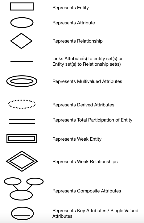
The Entity-Relationship (ER) model is a high-level data model that describes the real world as entities and the relationships between them. Its picture is the ER diagram, which serves as the blueprint for a database.

The ER notation used in the diagrams below.

Entity, entity set and attributes

Entity. A distinct real-world thing or object that exists physically, such as a college student, and can be uniquely identified by a primary attribute (the primary key).

• A strong entity can be identified on its own.
• A weak entity depends on a strong entity to exist and does not have enough attributes to be identified by itself. Take Loan (strong) and Payment (weak): payments are numbered 1, 2, 3 within each loan, so “payment 3” means nothing until you say which loan.

Entity set. A collection of entities of the same type that share the same attributes, such as Student, or Customer at a bank.

Attributes describe an entity. Each attribute takes its value from a set of allowed values called its domain. A Student entity might have Student_ID, Name, Standard, Course, Batch, Contact number and Address.

Types of attribute:

1. Simple: cannot be divided further. A customer’s account number, a student’s roll number.
2. Composite: can be split into parts. A person’s Name is first name, middle name and last name. Useful when you sometimes need the whole value and sometimes one part.
3. Single-valued: holds one value. Student ID, loan number.
4. Multivalued: holds more than one value, such as phone numbers or email addresses, often with a limit on how many.
5. Derived: computed from other attributes. Age, loan age, membership period.

NULL. An attribute is NULL when an entity has no value for it. NULL can mean “not applicable” (a person with no middle name) or “unknown” (a missing name, or an employee’s salary that has not been fixed yet).

Relationships

A relationship is an association among two or more entities: a person has a vehicle, a parent has a child, a customer borrows a loan.

• A strong relationship is between two independent entities.
• A weak relationship is between a weak entity and its owner, the strong entity. For example, Loan Payment.

Degree of a relationship is the number of entity sets taking part in it.

• Unary: one entity set. Employee manages Employee.
• Binary: two. Student takes Course.
• Ternary: three. Employee works-on Branch, Employee works-on Job.

Binary relationships are the common case.

Relationship constraints

1. Mapping cardinality (cardinality ratio). The number of entities another entity can be associated with through a relationship. With A and B as entity sets:

• One to one: an entity in A is associated with at most one entity in B, and an entity in B with at most one in A. Citizen has Aadhaar card.
• One to many: an entity in A is associated with N entities in B, and an entity in B with at most one in A. Citizen has Vehicle.
• Many to one: an entity in A is associated with at most one entity in B, and an entity in B with N entities in A. Course taken by Professor.
• Many to many: an entity in A is associated with N entities in B, and an entity in B with N entities in A. Customer buys Product.

2. Participation constraint (minimum cardinality).

1. Partial participation: not every entity takes part in the relationship.
2. Total participation: every entity must take part in at least one relationship instance.

In Customer borrows Loan, Loan has total participation, since a loan cannot exist without a customer. Customer has partial participation, since not every customer has a loan. A weak entity always has total participation; a strong entity may or may not.

---

Extended ER features

The basic ER features can model most databases. As the design grows more complex, the extended features below make the schema easier to express.

Specialisation

• Sometimes an entity set needs to be split into subgroups that differ from each other in some way.
• Specialisation splits an entity set into sub-entity sets based on their functions, specialities and features.
• It is a top-down approach.
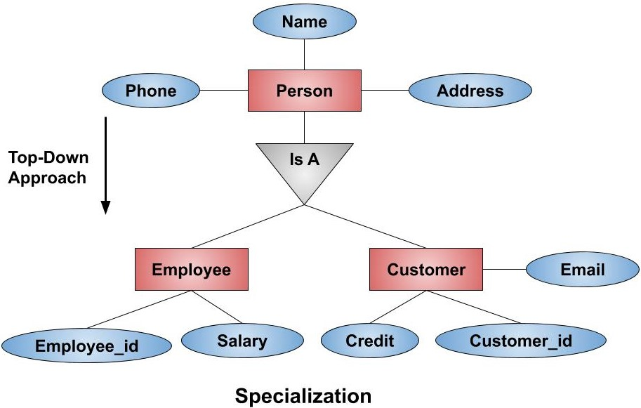
• Example: the Person entity set divides into Customer, Student and Employee. Person is the superclass and the others are subclasses.
  1. Superclass and subclass are joined by an is-a relationship.
  2. The ER diagram draws it as a triangle.

Specialisation: Person splits into Employee and Customer.

Why specialise?

• Some attributes apply only to some entities of the parent set.
• It lets the designer show what is distinctive about each sub-entity.
• Grouping those entities this way refines the whole design.

Generalisation

• The reverse of specialisation.
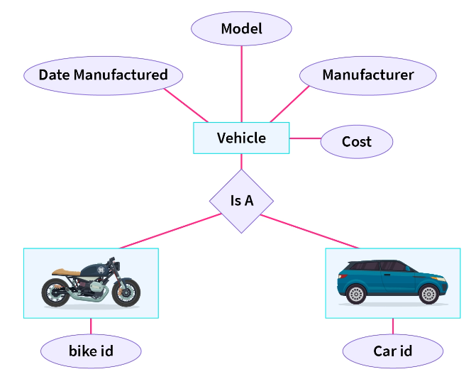
• A designer may notice that two entity sets share a lot of properties and decide to make a new, generalised entity set that becomes their superclass.
• Subclass and superclass are again joined by is-a.
• Example: Car, Jeep and Bus share many attributes. To avoid repeating them, the designer generalises them into a new entity set, Vehicle.
• It is a bottom-up approach.

Generalisation: bike and car roll up into Vehicle.

Why generalise?

1. The database becomes more refined and simpler.
2. Common attributes are not repeated.

Inheritance

• Attribute inheritance. Both specialisation and generalisation have it: lower-level entity sets inherit the attributes of higher-level ones. Customer and Employee inherit Person’s attributes.
• Participation inheritance. If a parent entity set takes part in a relationship, its child entity sets take part in it too.

Aggregation

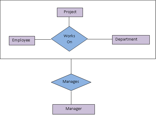
• How do you show a relationship among relationships? With aggregation.
• The relationship is abstracted and treated as a higher-level entity, an abstract entity.
• Treating the relationship as an entity set of its own avoids redundancy.

Employee works on Project in Department, and a Manager manages that whole arrangement.

---

Steps to make an ER diagram

The method is the same every time: gather requirements, find the entity sets, list their attributes and attribute types, then name the relationships with their mapping and participation constraints. Four worked examples follow.

Example: banking system

1. Requirements
   1. The banking system has branches (name is the primary key).
   2. The bank has customers.
   3. Customers hold accounts and take loans.
   4. A customer is assigned a banker.
   5. The bank has employees.
   6. Accounts are savings or current accounts.
   7. A loan is originated by a branch, is held by one or more customers, and has a payment schedule.
2. Entity sets
   1. Branch
   2. Customer
   3. Employee
   4. Savings account
   5. Current account
   6. Loan
   7. Payment (weak entity)
3. Attributes and their types
   1. Branch: name (PK), city, assets, liabilities
   2. Customer: cust-id (PK), name, address (composite), contact no. (multivalued), DOB, age (derived)
   3. Employee: emp-id (PK), name, contact no., dependent name (multivalued), years of service (derived), start date (single-valued)
   4. Generalised entity Account: acc-number (PK), balance
      1. Savings account: interest rate, daily withdrawal limit
      2. Current account: per-transaction charges, overdraft amount
   5. Loan: loan-number (PK), amount
   6. Payment (weak): payment no., date, amount
4. Relationships and constraints
   1. Customer Loan (M:N) [total participation]
   2. Loan Branch (N:1) [total participation]
   3. Loan Payment (weak) (1:N) [total participation]
   4. Customer Account (M:N) [partial participation]
   5. Customer Employee (N:1) [total participation]
   6. Employee Employee (N:1) [partial participation]

The banking ER diagram, drawn from the steps above.

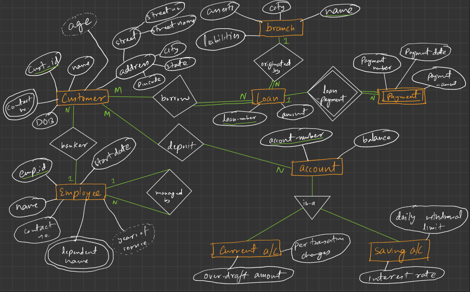
Example: online delivery system

1. Requirements
   1. The system has customers.
   2. Customers place orders and have addresses.
   3. Orders contain products.
   4. Customers have payment methods.
   5. The system has vendors.
   6. Vendors supply products.
   7. Orders go out for delivery.
2. Entity sets
   1. System
   2. Customer
   3. Order
   4. Address
   5. Product
   6. Payment method
   7. Vendor
   8. Delivery
3. Attributes and their types
   1. System: system_id (PK), name, version
   2. Customer: customer_id (PK), name, email, phone, registration_date
   3. Order: order_id (PK), order_date, total_amount
   4. Address: address_id (PK), street, city, state, postal_code
   5. Product: product_id (PK), name, description, price
   6. Payment method: payment_id (PK), method_type, card_number, expiration_date
   7. Vendor: vendor_id (PK), name, email, phone
   8. Delivery: delivery_id (PK), delivery_date, status
4. Relationships and constraints
   1. Customer Order (1:N) [total participation]
   2. Order Product (M:N) [partial participation]
   3. Customer Payment method (M:N) [partial participation]
   4. Customer Address (1:N) [total participation]
   5. Vendor Product (1:N) [total participation]
   6. Order Delivery (1:1) [partial participation]

A close relative of the delivery model: an online pizza-ordering system, where the products are pizzas and non-pizza items built from ingredients.

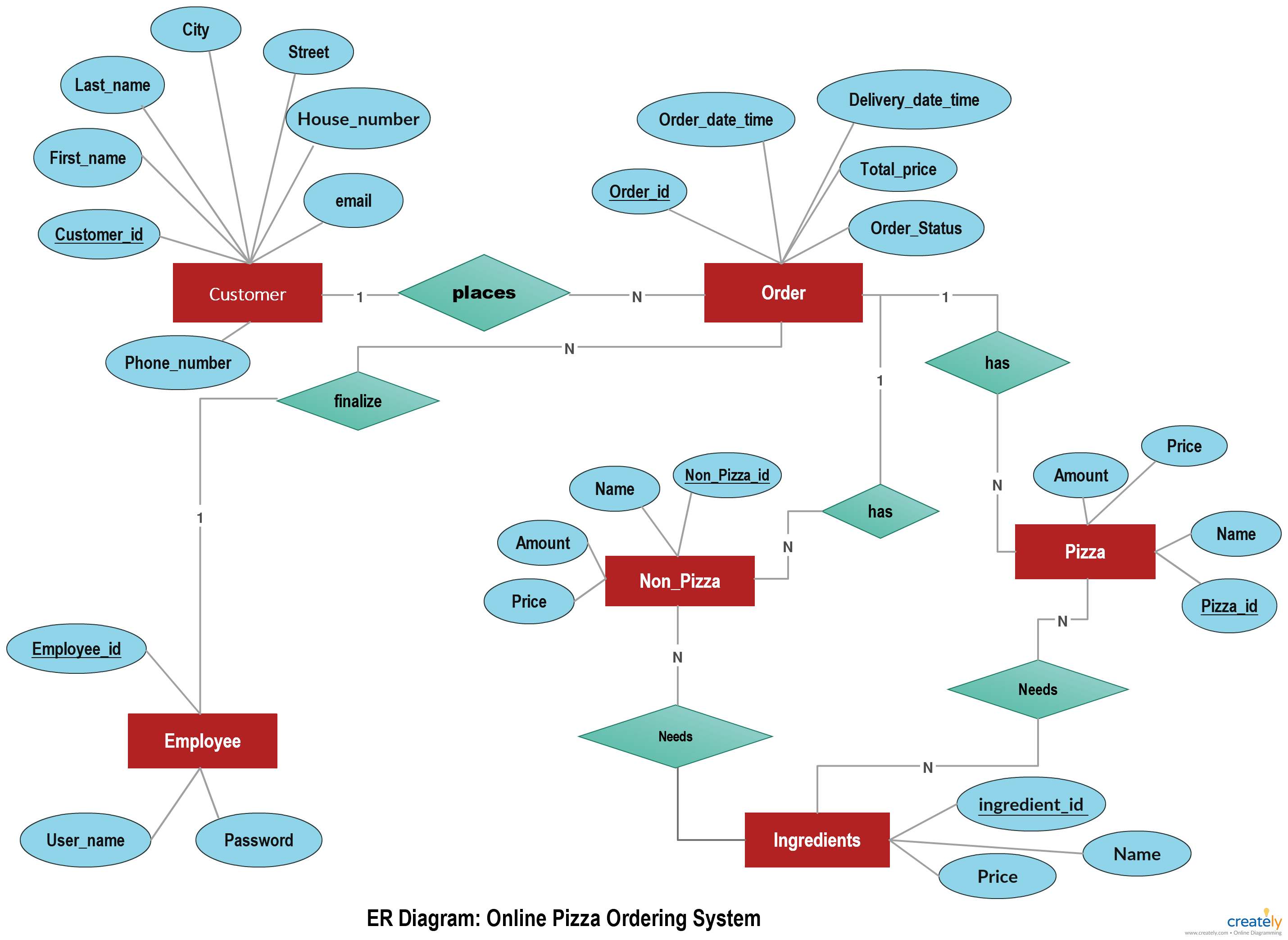
Example: university

1. Requirements
   1. The university has departments (name is the primary key).
   2. Departments offer courses.
   3. Students take courses.
   4. Students enrol and take exams.
   5. Each student has a faculty advisor.
   6. Faculty teach courses.
   7. Courses have prerequisites.
   8. Exams follow an exam schedule.
2. Entity sets
   1. University
   2. Department
   3. Course
   4. Student
   5. Faculty
   6. Exam
   7. Enrollment (weak entity)
   8. Prerequisite (weak entity)
   9. Exam schedule
3. Attributes and their types
   1. University: name (PK), location, founding year, contact info
   2. Department: name (PK), head of department, office location
   3. Course: code (PK), title, credits, syllabus
   4. Student: student-id (PK), name, address, contact no., DOB, age (derived)
   5. Faculty: faculty-id (PK), name, specialisation, office location, contact no.
   6. Exam: exam-id (PK), date, time, location
   7. Enrollment (weak): enrollment-id (PK), enrollment date
   8. Prerequisite (weak): prerequisite-course-code (PK)
   9. Exam schedule: schedule-id (PK), exam date, start time, end time, location
4. Relationships and constraints
   1. Student Course (M:N) [partial participation]
   2. Course Department (N:1) [total participation]
   3. Student Exam (M:N) [partial participation]
   4. Course Prerequisite (1:N) [total participation]
   5. Faculty Student (1:N) [total participation]
   6. Faculty Course (M:N) [partial participation]
   7. Department Faculty (N:1) [partial participation]
   8. Exam Course (1:N) [total participation]

The core of that, as an entity-relationship sketch:

flowchart LR
    Dept[Department] ---|offered by · N:1| Course[Course]
    Dept ---|headed by · N:1| Fac[Faculty]
    Fac ---|teaches · M:N| Course
    Fac ---|advises · 1:N| Stu[Student]
    Stu ---|enroll · M:N| Course
    Stu ---|takes · M:N| Exam[Exam]
    Exam ---|scheduled for · 1:N| Course
    Course ---|has prerequisites · 1:N| Pre[[Prerequisite · weak]]
    classDef gateway fill:#EDE9FE,stroke:#7C3AED,color:#4C1D95,stroke-width:2px
    classDef warn    fill:#FEF3C7,stroke:#D97706,color:#78350F,stroke-width:2px
    class Dept,Course,Fac,Stu,Exam gateway
    class Pre warn

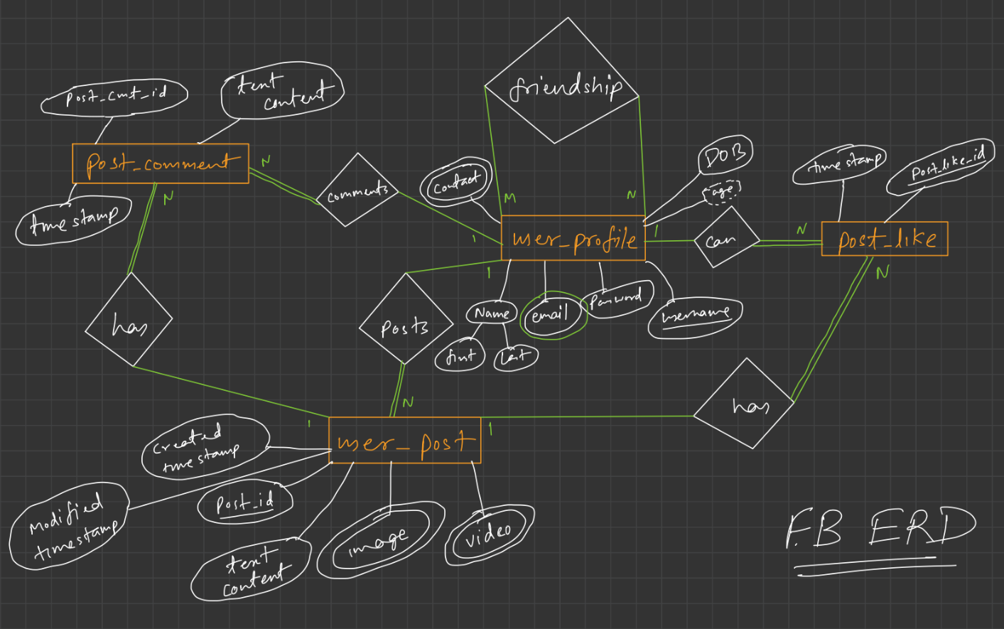
Example: a Facebook-like social network

1. Requirements
   1. The platform has users.
   2. Users write posts and comments.
   3. Users form friendships.
   4. Users send messages.
   5. Users follow pages.
   6. Posts get likes and tags.
   7. Pages publish posts.
2. Entity sets
   1. User
   2. Post
   3. Comment
   4. Friendship
   5. Message
   6. Page
   7. Like (weak entity)
   8. Tag (weak entity)
3. Attributes and their types
   1. User: user-id (PK), username, email, date of birth, gender, profile picture, bio
   2. Post: post-id (PK), content, timestamp
   3. Comment: comment-id (PK), text, timestamp
   4. Friendship: friendship-id (PK), user1-id (FK), user2-id (FK), status
   5. Message: message-id (PK), sender-id (FK), receiver-id (FK), content, timestamp
   6. Page: page-id (PK), page name, description
   7. Generalised entity Interaction: interaction-id (PK), user-id (FK), timestamp
      1. Like (weak): post-id (FK), interaction-id (FK)
      2. Tag (weak): post-id (FK), interaction-id (FK)
4. Relationships and constraints
   1. User Post (1:N) [total participation]
   2. User Comment (1:N) [total participation]
   3. User Message (1:N) [total participation]
   4. User User (M:N) [partial participation]
   5. User Post (M:N) [partial participation]
   6. User Post (M:N) [partial participation]
   7. User Page (M:N) [partial participation]
   8. Page Post (1:N) [total participation]

A trimmed version drawn by hand: user profiles, posts, comments, likes and friendships. The relational section below turns this diagram into tables.

---

The relational model

What is the relational model?

• The relational model (RM) organises data into relations, which are tables. A relational database is a set of uniquely named tables, and each row in a table records a relationship among a set of values.
• A tuple is one row: a single record.
• A column is an attribute of the relation, and each attribute has a domain of allowed values.
• The relation schema is the design of the relation: its name and all its columns.
• DBMSs built on the relational model are called RDBMSs. Oracle, IBM Db2, MySQL and MS Access are common ones.

Degree and cardinality

• Degree of a table: its number of attributes (columns).
• Cardinality: its number of tuples (rows).

Properties of a table

• Every relation has a name distinct from all other relations.
• Values are atomic: they cannot be broken down further.
• Every attribute (column) name within a relation is unique.
• Every tuple is unique.
• The order of rows and columns carries no meaning.
• Tables follow integrity constraints, which keep data consistent across tables.

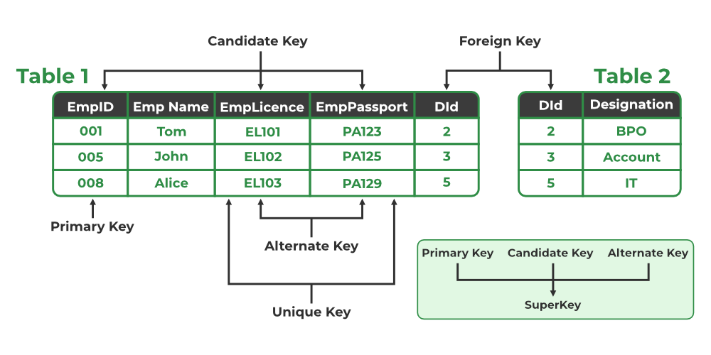
Keys

A relational key is a set of attributes that uniquely identifies each tuple.

1. Super key (SK): any combination of attributes that uniquely identifies each tuple.
2. Candidate key (CK): a minimal super key: one that still identifies each tuple but has no redundant attribute. A CK value cannot be NULL.
3. Primary key (PK): the candidate key chosen to identify rows, usually the one with the fewest attributes.
4. Alternate key (AK): every candidate key that was not chosen as the PK.
5. Unique key: a key that enforces unique values across its attribute(s).
6. Foreign key (FK):
   • Creates a relation between two tables.
   • A relation r1 may include among its attributes the PK of another relation r2. That attribute is a foreign key from r1 referencing r2.
   • r1 is the referencing (child) relation of the dependency, and r2 is the referenced (parent) relation.
   • Foreign keys are how you cross-reference between two relations.
7. Composite key: a PK made of at least two attributes.
8. Compound key: a PK made of two foreign keys.
9. Surrogate key:
   1. A synthetic PK.
   2. Generated automatically by the database, usually an integer.
   3. Can be used as the PK.

The keys on one example. Primary, candidate and alternate keys are all super keys.

Integrity constraints

• CRUD operations have to follow an integrity policy so the database is always consistent.
• The constraints exist so you do not corrupt the database by accident.

Domain constraints

• Restrict the values an attribute can take, i.e. specify its domain.
• Restrict the data type of every attribute.
• Example: enrolment should only be allowed for candidates born before 2002.

Entity constraints

• Every relation must have a PK, and the PK cannot be NULL.

Referential constraints

• Defined between two relations, they keep the tuples of the two consistent with each other.
• Insertion constraint: a value in the referencing relation’s specified attributes must also appear in the specified attributes of at least one tuple in the referenced relation.
• Deletion constraint: if an FK in the referencing table points to the PK of the referenced table, every FK value must be NULL or present in the referenced table. So you cannot delete a parent row while children still point to it.
• In short: every FK value must have a matching PK in the parent table, or be NULL.

Can you delete a parent row whose value is still used in the child table, without breaking the deletion constraint? Two options:

• ON DELETE CASCADE: deleting the parent row automatically deletes the child rows that reference it.
• ON DELETE SET NULL: this also answers “can an FK be NULL?” Yes. When the parent row is deleted, the child rows’ FK values are set to NULL. Referential integrity holds and nothing cascades.

Key constraints

1. NOT NULL: the column cannot hold NULL, so every row has a value for it.
2. UNIQUE: every value in the column is different from every other.
3. DEFAULT: sets a default value, used when an insert gives none.
4. CHECK: an integrity constraint that keeps data valid before and after each CRUD operation.
5. PRIMARY KEY: an attribute or set of attributes that uniquely identifies each entity. Values must be unique and not NULL.
6. FOREIGN KEY: when two entities are related, they share an attribute. That attribute is the PK of one entity set and becomes a foreign key in the other. The FK blocks any action that would break the link between the tables.

From ER model to relational model

The ER model and the relational model are both abstract, logical representations of a real enterprise, and they follow similar design principles. So an ER design can be converted into a relational design: turning each piece of the ER diagram into tables is how you get from the diagram to a relational schema.

How each ER construct becomes a relation:

1. Strong entity
   • Becomes its own table named after the entity; its attributes become columns.
   • The entity’s PK becomes the relation’s PK.
   • FKs are added to link it to other relations.
2. Weak entity
   • Becomes a table with all the entity’s attributes.
   • The PK of its owning strong entity is added as an FK.
   • The PK is composite: {FK + partial discriminator key}.
3. Single-valued attributes
   • Become columns directly.
4. Composite attributes
   • Each component becomes its own column in the original relation, and the composite itself is dropped.
   • Example: Address {street-name, house-no} on Customer becomes two columns, address_street_name and address_house_no, and there is no Address column.
5. Multivalued attributes
   • Each multivalued attribute gets a new table, named after the attribute.
   • The entity’s PK goes into the new table as an FK.
   • A column holding the attribute’s values is added.
   • The new table’s PK is {FK + value column}.
   • Example: Employee has the multivalued attribute dependent-name. A new table dependent_name is created with columns emp_id and dname; PK {emp_id, dname}; FK {emp_id}.
6. Derived attributes are not stored in tables.
7. Generalisation
   • Method 1: create a table for the higher-level entity set. For each lower-level entity set, create a table with a column for each of its own attributes plus a column for each attribute of the higher-level set’s primary key. For the banking Account generalisation:
     1. account (account_number, balance)
     2. savings_account (account_number, interest_rate, daily_withdrawal_limit)
     3. current_account (account_number, overdraft_amount, per_transaction_charges)
   • Method 2: if the generalisation is disjoint (no entity belongs to two lower-level sets) and complete (every higher-level entity belongs to some lower-level set), skip the higher-level table. Each lower-level table gets its own attributes plus all the higher-level attributes:
     1. savings_account (account_number, balance, interest_rate, daily_withdrawal_limit)
     2. current_account (account_number, balance, overdraft_amount, per_transaction_charges)
   • Drawbacks of method 2: on an overlapping generalisation, values such as balance would be stored twice. On an incomplete one, an account that is neither savings nor current has no table to live in.
8. Aggregation
   • Make a table for the relationship set.
   • Its columns are the primary keys of the entity set and of the entities inside the aggregation.
   • Add any descriptive attributes the relationship has.
9. Unary relationships
   • Create a new table for the relationship, with a column for the entity’s PK and an FK back to the same entity.
   • For “supervises”, make an Employee_Supervises table with employee_id (FK) and supervisor_id (also an FK).
   • The two IDs together form the PK, so each supervisory link appears once.

Facebook: from ER diagram to tables

Applying those rules to the hand-drawn Facebook diagram above gives nine relations. Underlined columns in the original drawing are the key; here the key is listed first.

#	Relation	Columns
1	user_profile	username, name_first, name_last, password, DOB
2	user_profile_email	username (FK), email
3	user_profile_contact	username (FK), contact_number
4	friendship	profile_req (FK), profile_accept (FK), a compound key
5	post_like	post_like_id, timestamp, post_id (FK), username (FK)
6	user_post	post_id, created_timestamp, modified_timestamp, text_content, username (FK)
7	user_post_image	post_id (FK), image_url
8	user_post_video	post_id (FK), video_url
9	post_comment	post_comment_id, text_content, timestamp, post_id (FK), username (FK)

Email and contact are multivalued, so they became tables 2 and 3 (rule 5). Image and video on a post are multivalued too, so they became 7 and 8. Age was derived, so it is gone (rule 6). Friendship is a unary M:N relationship on user_profile, so it became its own table whose key is two foreign keys (rule 9, and a compound key from the key list).

---

That is the design side: from raw facts to a schema. The next part writes that schema, and queries it, in SQL.

Next: SQL, from CREATE TABLE to fifty interview queries

dbms databases er-model relational-model series